If you google “single line python server” you can find many references to SimpleHttpServer implementation of python. This is really useful for testing a remote http server
in your local machine by changing output of the service as you wish.
It’s usage is really simple, so you can start the web server by typing the following command :
> python -m SimpleHTTPServer 8000
Now you have a web server on your local machine listening on port 8000. You can test it by using the url below in your browser :
> http://127.0.0.1:8000
The directory that you run the command is the root of your web server. You can put a simple json file into this directory and return it against your http “get” calls by adding this json file
into your url :
> http://127.0.0.1:8000/result.json
The restriction of this simple http server is that you can use only “get” method for your http calls. If you try to send post requests, you will get the following or any similar error on the console.
> code 501, message Unsupported method ('POST')
Let’s add “post” method support to the SimpleHttpServer. The following python
script inherits SimpleHttpServer and adds do_POST method for simulating post http calls.
Please read my previous blog post about SVD(Singular Value Decomposition) if you are not familiar with.
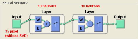
Neural Network Structure
I have used simple feed-forwarding back-propagation neural network. Because most important part here is pre-processing step which I have applied SVD method for reducing dimension as input size of the neural network.
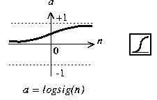
There are two layers which has 10 neurons. Input size of network is 7 x 5 = 35 which means pixel count of character. I have used “logsig” transfer function for obtaining values between 0 and 1.
Because there are 10 output neurons in network which means 10 digit. The biggest value of these 10 output neurons is accepted as digit to be learned or recognized.
I have used “traingdx” variable of matlab for providing gradient descent backpropagation with adaptive learning rate. I have used SSE (Sum of squared error) as performance measure. Neuron weights are determined randomly. Error rate is determined as “0.1” which means training will continue until error rate reached to this value. Epoch size is determined as 50000 but training cycles never reach to this value, because the size of my training set is small. I have using 40 characters for training and 10 for test. Momentun constant which is used in back propagation is 0.95.
Using SVD(Singular Value Decomposition)
As I have mentioned on the previous parts, SVD is used to reduce dimension and uncorrelate correlated data which means feature extraction. In this project I have sampled text classification method which is mentiond in [2]. As similar to [term x document] model which is generally used in LSA (Latent Semantic Analysis), I have created [pixel x character] space.
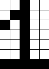
On image processing part of this project, I have cropped characters from bitmap image and stretched the size of images to 7 x 5 pixel.
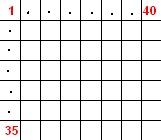
For obtaining pixel X character matrix, I have convetred this image into column vector form. (35 x 1). I have 40 characters in my training set which provides 35 x 40 matrix as [pixel x character] matrix.
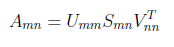
This is our A matrix which we will use in SVD part. We have added all training data into our matrix, because we will consider all possible values and its correlations for obtaining good features and suppress the noise. I have applied SVD method to this matrix and obtained 3 matrices of SVD.
After obtaining U [35x35],S[35x40] and V[40x40] matrices, we can try to reduce dimension. There are 35 singular values in S matrix and most important ones are on the top. In U matrix columns vectors are orthonormal which means as uncorrelated as possible. We know that the vectors contain components ordered from most to least amount of variation accounted for in the original data. By deleting elements representing dimensions which do not exhibit meaningful variation, we efectively eliminate noise in the representation of pixel vectors.
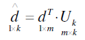
Let say we have determined to use only 30 of 35 column vectors in U. In this case last 5 columns are removed. Then we will multiply all characters in training data set with this new dimension reduced U matrix.
In this equation m is our original dimension value “35”, k is the reduced dimension value “30”. Transpose of d is our original character input vector exists in training data set. New d parameter is our dimension reduced input value. By making this multiplication, we are extracting most important features of character and suppress noise. Additionally we use less input values which will decrease the testing in real time applications.
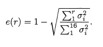
For determining reduced dimension, I have used following formula which is explained in [1].
By setting an error threshold value, we can use the above equation for determining “r” value which is reduced size of singular values. In my project, I set the error threshold as “0.05”. Now the pixel vectors are shorter, and contain only the elements that account for the most significant correlations among pixels in the original dataset.
Experimental Results
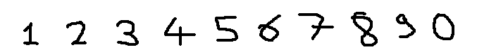
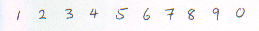
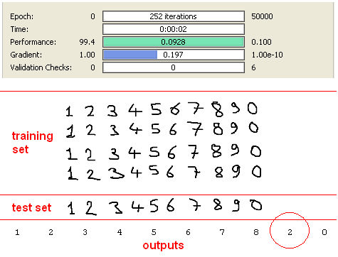
I have used 3 different training and test sets in my experiments. Two handwritten data and one predefined font. All data sets contain 40 training and 10 test data. Example view of data sets are seen as below.
First data set :
Second data set :
Third data set :
We will begin with the first data set which I have created using ms paint application :)
First Data Set
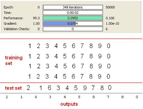
I have executed my application with default parameter values, but training process taked long time and I have cancelled the process. Because all of 40 characters are the same in the training set.
So, after applying SVD considering 0.05 error rate, dimension is reduced to 3 from 35. This is possible if training data is not correlated and without noise. But in this case Neural Network training process will be longer, because it is not easy to classify 10 classes with only 3 inputs. After observing this behavior, I have determined to reduce error Threshold to “0.01” for getting reduced dimension greater than 3.After this improvement, I have obtained “7” as new dimension and also input size of neural network. Results are seen in the following screen shot.
As expected, this result is very good, because training set and test set are the same. But it should be considered that this achievement is provided only using 7 inputs.
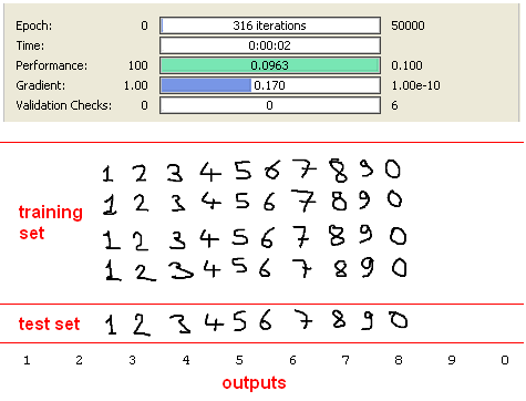
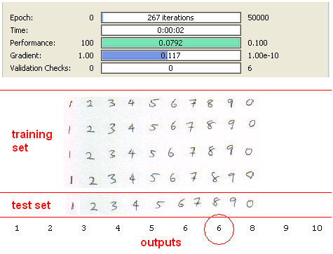
On the other hand, if we execute the application without using SVD preprocessing method by applying 35 inputs the results are shown below.
There are not so big difference between iteration counts and SVD approach really works if we consider 5 times reduced dimension of input.
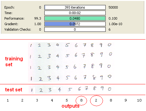
Second Data Set
Second data set consists of handwritten digits created by using mouse on ms paint application. This data set is more correlated than the first one and there are some noisy pixels arround characters due to distortion while using mouse. But results with SVD are great again with using only 8 inputs instead of 35.
I have used same data set without SVD preprocessing step and obtained following results.
As we can see in results figure, “9” character is recognised as “2”. After this result, we can say that SVD method really suppress the noise on the original data while reducing dimension.
Third Data Set
Third data set consist of handwritten and scanned paper. Results with SVD is seen as below.
Digit “7” is recognised as “6” due to small size of training data. This problem can be prevented by using bigger training data. Anyway, %90 is a good achievement with only “8” inputs again.
Without SVD results are seen as below.
Success rate is %80 which is less than SVD preprocessing approach.
Conclusion
I have applied vector-space model commonly used in text-classification into my optical digit recognition project. According to experiments, SVD recudes the dimension drastically, suppress the noise and provide us uncorrelated data set which is easier to differentiate. So, recognizing performance of SVD is better than standart method. If the original data set has gigantic amount of dimension, SVD method can provide really good improvement for decreasing training time.
[1] “A Singular Value Decomposition: The SVD of a Matrix”, Dan Kalman, January – [1996]
[2] “Neural Network for Text Classification Based on Singular Value Decomposition”, Cheng Hua Li and Soon Cheol Park, “IEEE Sevent International Conference on Computer and Informaiton Technology”, University of Aizu, Fukushima Japan, October 16 to 19, [2007]
Singular Value Decomposition can be seen as a feature extraction method which transforms correlated variables into a set of uncorrelated ones that better expose relationships on the original data.
On the other hand, it is possible to determine dimension along which data points shows the most variation. It is possible find best approximation of the original data by reducing dimension.
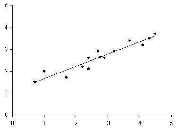
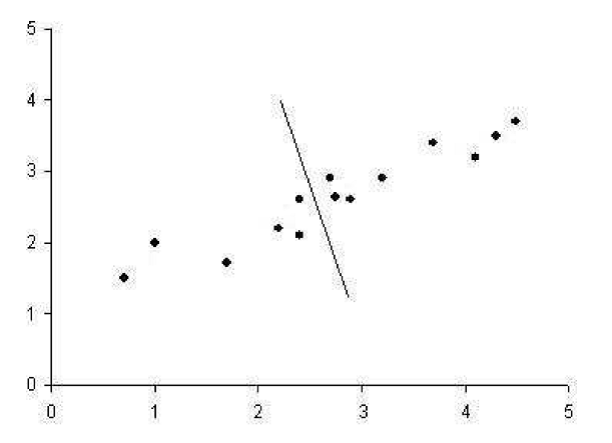
There are 2 dimensional data points in the following figure which regression line running through them shows the best approximation of the original data.
In this classification, inner class differences are small, and between class differences are big. If we draw perpendicular line from each point to the regression line, and took the intersection of those lines as the approximation of the original data point, we would have a reduced representation of the original data that captures as much of the original variation as possible.
Second regression line which is perpendicular to first one gives poor result for approximating the original data.
It captures as much of the variation as possible along the second dimension of the original data set.
It is possible to use these regression lines to generate a set of uncorrelated data points that will show subgroupings in the original data not necessarily visible at first glance. SVD reduces the high dimensional, highly variable set of data points to a lower dimensional space that exposes the substructure of the original data more clearly and orders it from most variation to the least.
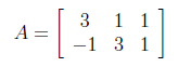
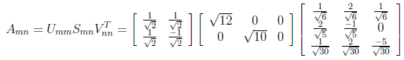
From linear algebra point of view, we have “A” rectangular matrix which can be divided into product of three matrices are orthogonal “U”, diagonal “S”, transpose of orthogonal “V”.
In the above equation, U^T U=I and V^T V=I. The columns of U are orthonormal eigenvectors of AA^T , the columns of V are orthonormal eigenvectors of A^T A and S is the diagonal matrix containing the square roots of eigenvalues from U or V in descending order.
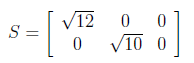
SVD of an example matrix
We have 3x2 rectangular matrix decomposing to its singular values.
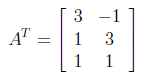
For finding U from AA^T , first we need to calculate transpose of A as below.
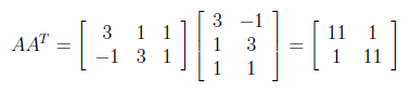
After finding transpose of A, AA^T can be found as follows.
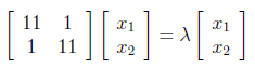
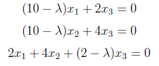
Next, we have to find the eigenvalues and corresponding eigenvectors of AA^T . We know that eigenvectors are defined by the equation , and applying this to AA^T gives us :
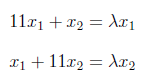
We can write above matrix equation as set of equations as below
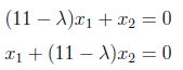
and can equal to “0” as follows.
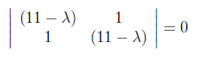
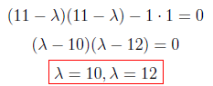
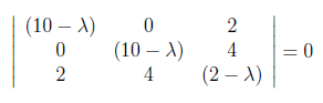
For finding λ values, we have to set to zero the determinant of the coefficient matrix.
After making the multiplications we found λ values as “10” and “12” as below.
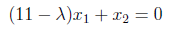
In this step, we will put λ values back in the following equation and find eigenvectors.
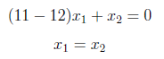
For λ = 10 :
Now, the above equation is true for lots of values, we will select simplest ones and easiest to work with. So x1 = 1, x2 = -1. We obtained the eigenvector for λ=10 as [1 -1].
For λ = 12 :
As similar to previous case we have obtained x1 = 1 and x2 = 1. So eigenvector of λ=12 is [1 1]. These eigenvectors become column vectors in a matrix ordered by the size of the corresponding eigenvalue. In other words, the eigenvector of the largest eigenvalue is column one, the eigenvector of the next largest eigenvalue is column two, and so forth and so on until we have the eigenvector of the smallest eigenvalue as the last column of our matrix.
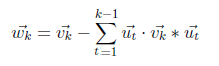
The above 2x2 matrix is initial matrix of U. Now we will try to obtain an orthogonal matrix by using this initial matrix. This initial matrix contains eigenvectors of AA^T. But we have to find orthonormal eigenvectors of AA^T for generating U matrix. There are several methods for orthonormalization and I have used Gram-Schmidt method. It basically begins by normalizing the first column vector under consideration and iteratively rewriting the remaining vectors in terms of themselves minus a multiplication of the already normalized vectors.
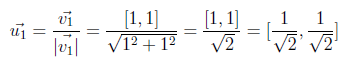
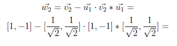
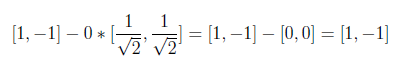
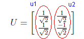
Begin normalization with [1 1] vector belongs to λ=12.
Now we will compute w2 by using the above formula.
In the following equation, “0” on the left side comes from inner product and result is found as [1 -1].
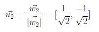
On the last step, we will normalize second vector by using w2 as below.
Now we have u1 and u2 northonormal vectors and U matrix is generated as shown in the following figure.
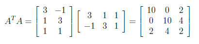
As similiar to finding U matrix, now we will calculate A^T A for generating V orthogonal matrix.
V matrix is generated as below by applying the same steps which we have followed for obtaining U matrix.
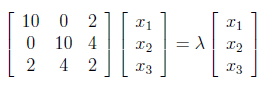
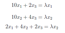
Above matrix equation form represents the system of equations
which write as
which are solved by setting
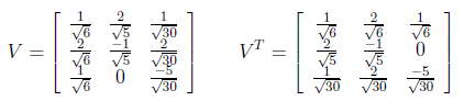
After applying same steps used while obtaining U, λ values are found as “0”, “10” and “12” and initial V matrix which consist of eigenvectors of A^T A is shown as below.
After Gram-Schmidt Orthonormalization process, V matrix and its transpose are found as below.
The last member of SVD decomposition is S orthogonal matrix which consist of square roots of eigen values. The non-zero eigenvalues of U and V are always the same, so that’s why it doesn’t matter which one we take them from.
Finally A matrix can be written as divided into 3 matrix in the following figure.
I hope you are still with me!. I will share another blog post next week about how to use SVD as pre-process of Neural Networks for improving the recognition performance and reducing input space dimension.
If you are using Parse backend in one of your application/game like me, you already sadly know that Parse’s backend services will be fully retired on January 28, 2017 and you probably started to migrate your data and cloud code to an
alternative db and backend service.
I have already started to migration process and decided to try MongoLab and AWS. Before to deploy our cloud code to AWS, I set up parse server environment on my local computer and running parse service succesfully. Problem is that when I call
Parse.Promise.when() with multiple commands like that :
it returns different result than I am getting from parse servers. Difference is that returning json object on my local computer has only one key as “0” and an object array
as value.
I firstly suspect that MongoDB configurations are different and that’s why the data has been retrieved in different format and
saw this doesn’t make sense after 30 minutes of investigation.
Here, “promises” is input queriy you pass into Parse.Promise.when() and you can see that if your input is an array, so consist of multiple queries, then square brackets are applied to returning object. This code change is commited
on December 10, 2015 and reverted on January 09, 2016 with this revert commit.
For resolving this issue, I have downloaded the latest Parse JS SDK and replaced ParsePromise.js with up to date version.
If you are from java world like me, you most probably have chained methods using simple static builder class while instantiating your objects and you know this is builder pattern in aspect of chaining.
In one of our ndk-android game projects I decided to implement chaining rule of builder pattern instead of using classical “getter/setter” usage. Additionally I was
planning to use native heap instead of usign local stack memory and I didn’t want to use any friend classes which I don’t find so natural.
I just wanted to instantiate a builder and build my actual object on it. But here, we have to pay attention to possible memory leaks and remove our builder instance on deconstructor of actual object. In the light
of these requirements I have implemented my “GiftModel” class as follows.