
Singular Value Decomposition can be seen as a feature extraction method which transforms correlated variables into a set of uncorrelated ones that better expose relationships on the original data. On the other hand, it is possible to determine dimension along which data points shows the most variation. It is possible find best approximation of the original data by reducing dimension.
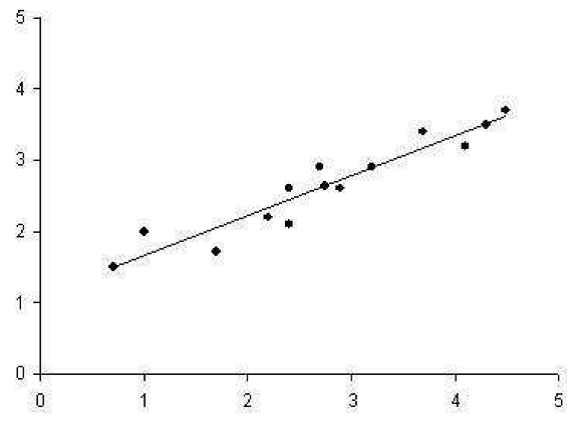
There are 2 dimensional data points in the following figure which regression line running through them shows the best approximation of the original data. In this classification, inner class differences are small, and between class differences are big. If we draw perpendicular line from each point to the regression line, and took the intersection of those lines as the approximation of the original data point, we would have a reduced representation of the original data that captures as much of the original variation as possible.
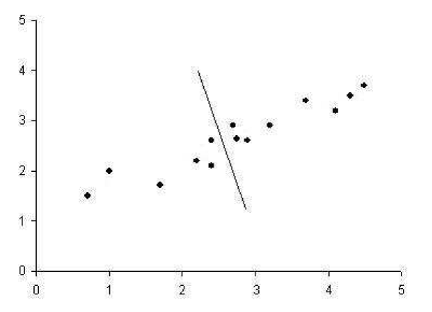
Second regression line which is perpendicular to first one gives poor result for approximating the original data. It captures as much of the variation as possible along the second dimension of the original data set.
It is possible to use these regression lines to generate a set of uncorrelated data points that will show subgroupings in the original data not necessarily visible at first glance. SVD reduces the high dimensional, highly variable set of data points to a lower dimensional space that exposes the substructure of the original data more clearly and orders it from most variation to the least.
From linear algebra point of view, we have “A” rectangular matrix which can be divided into product of three matrices are orthogonal “U”, diagonal “S”, transpose of orthogonal “V”.
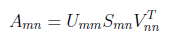
In the above equation, U^T U=I and V^T V=I. The columns of U are orthonormal eigenvectors of AA^T , the columns of V are orthonormal eigenvectors of A^T A and S is the diagonal matrix containing the square roots of eigenvalues from U or V in descending order.
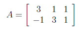
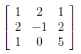
SVD of an example matrix
We have 3x2 rectangular matrix decomposing to its singular values.
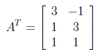
For finding U from AA^T , first we need to calculate transpose of A as below.
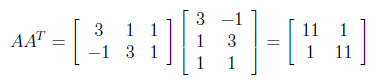
After finding transpose of A, AA^T can be found as follows.
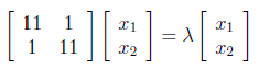
Next, we have to find the eigenvalues and corresponding eigenvectors of AA^T . We know that eigenvectors are defined by the equation , and applying this to AA^T gives us :
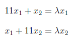
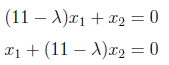
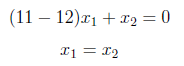
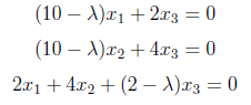
We can write above matrix equation as set of equations as below
and can equal to “0” as follows.
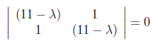
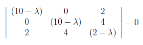
For finding λ values, we have to set to zero the determinant of the coefficient matrix.
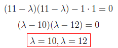
After making the multiplications we found λ values as “10” and “12” as below.
In this step, we will put λ values back in the following equation and find eigenvectors.
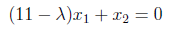
For λ = 10 :

Now, the above equation is true for lots of values, we will select simplest ones and easiest to work with. So x1 = 1, x2 = -1. We obtained the eigenvector for λ=10 as [1 -1].
For λ = 12 :
As similar to previous case we have obtained x1 = 1 and x2 = 1. So eigenvector of λ=12 is [1 1]. These eigenvectors become column vectors in a matrix ordered by the size of the corresponding eigenvalue. In other words, the eigenvector of the largest eigenvalue is column one, the eigenvector of the next largest eigenvalue is column two, and so forth and so on until we have the eigenvector of the smallest eigenvalue as the last column of our matrix.

The above 2x2 matrix is initial matrix of U. Now we will try to obtain an orthogonal matrix by using this initial matrix. This initial matrix contains eigenvectors of AA^T. But we have to find orthonormal eigenvectors of AA^T for generating U matrix. There are several methods for orthonormalization and I have used Gram-Schmidt method. It basically begins by normalizing the first column vector under consideration and iteratively rewriting the remaining vectors in terms of themselves minus a multiplication of the already normalized vectors.
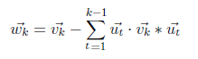
Begin normalization with [1 1] vector belongs to λ=12.
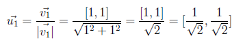
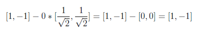
Now we will compute w2 by using the above formula.
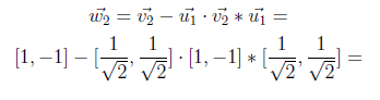
In the following equation, “0” on the left side comes from inner product and result is found as [1 -1].
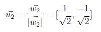
On the last step, we will normalize second vector by using w2 as below.
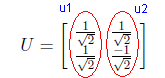
Now we have u1 and u2 northonormal vectors and U matrix is generated as shown in the following figure.
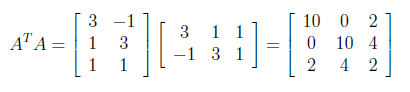
As similiar to finding U matrix, now we will calculate A^T A for generating V orthogonal matrix.
V matrix is generated as below by applying the same steps which we have followed for obtaining U matrix.
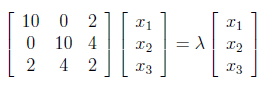
Above matrix equation form represents the system of equations
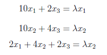
which write as
which are solved by setting
After applying same steps used while obtaining U, λ values are found as “0”, “10” and “12” and initial V matrix which consist of eigenvectors of A^T A is shown as below.
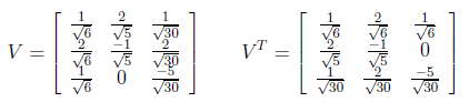
After Gram-Schmidt Orthonormalization process, V matrix and its transpose are found as below.
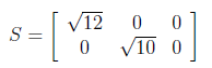
The last member of SVD decomposition is S orthogonal matrix which consist of square roots of eigen values. The non-zero eigenvalues of U and V are always the same, so that’s why it doesn’t matter which one we take them from.
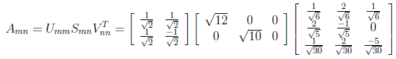
Finally A matrix can be written as divided into 3 matrix in the following figure.
I hope you are still with me!. I will share another blog post next week about how to use SVD as pre-process of Neural Networks for improving the recognition performance and reducing input space dimension.